3 - PyTorch Basics
In this section we will explore some of the basics of PyTorch. We won't go into too much detail, but we will cover the most important concepts. If you want to learn more about PyTorch, you can check the official documentation (opens in a new tab). We also linked additional useful resources throughout the guide.
You can find a full PyTorch example at example.py.
3.1 - Tensor
The basic data structure in PyTorch is the tensor, a multi-dimensional array, similar to NumPy's np.ndarray. This is the data structure that you will use to store data, variables, model parameters and gradients.
Full PyTorch Tensor documentation is available in this page (opens in a new tab).
3.1.1 - Tensor Creation
Tensors can be created in several different ways. Namely:
-
Using the
torch.tensorfunction. The code below, for example, creates a tensor with 3 rows and 2 columns.import torch x = torch.tensor([[1, 2], [3, 4], [5, 6]]) -
From a NumPy array
x_numpy = np.array([[1, 2], [3, 4]]) x_torch = torch.from_numpy(x_numpy) -
With constant data
x = torch.ones(2, 3) # 2 rows and 3 columns of ones y = torch.zeros(3, 2) # 3 rows and 2 columns of zeros -
With random data
x = torch.rand(2, 3) # uniform distribution U(0, 1) y = torch.randn(2, 3) # standard gaussian N(0, 1) z = torch.randint(0, 10, size=(2, 3)) # random integers [0, 10) -
Others
torch.arange(5)  # from 0 (inclusive) to 5 (exclusive)
torch.arange(2, 8)  # from 2 to 8
torch.arange(2, 8, 2)  # from 2 to 8, with stepsize=2

torch.linspace(0, 1, 6)  # returns 6 linear spaced numbers from 0 to 1 (inclusive)
torch.linspace(-1, 1, 8)  # returns 8 linear spaced numbers form -1 to 1

torch.eye(3)  # identity matrix
3.1.2 Tensor Data Types
When creating a tensor, you can specify the data type with the dtype argument.
x = torch.ones(2, 3, dtype=torch.float32)You can also change the data type of an existing tensor with the tensor.type() method.
x = torch.ones(2, 3, dtype=torch.float32)
x.type(torch.float64)
The following table shows some of the main data types supported by PyTorch. The full list of data types supported by PyTorch is available in the official documentation (opens in a new tab).
| Data type | Description |
|---|---|
torch.float64 | 64-bit floating point |
torch.float32 | 32-bit floating point |
torch.float16 | 16-bit floating point |
torch.bfloat16 | 16-bit floating point |
torch.int64 or torch.long | 64-bit integer |
torch.int32 or torch.int | 32-bit integer |
torch.int16 or torch.short | 16-bit integer |
torch.int8 | 8-bit integer |
torch.uint8 | 8-bit unsigned integer |
torch.bool | Boolean |
3.1.3 - Tensor Operations
The following table shows some of the most common tensor operations. For a full and updated list, please refer to the official documentation (opens in a new tab).
| Operation | Description |
|---|---|
x + y | Element-wise addition |
x - y | Element-wise subtraction |
x * y | Element-wise multiplication |
x / y | Element-wise division |
x @ y | Matrix multiplication |
x.T | Transpose |
x.sum() | Sum of all elements |
x.mean() | Mean of all elements |
x.std() | Standard deviation of all elements |
x.min() | Minimum value of all elements |
x.max() | Maximum value of all elements |
x.abs() | Absolute value of all elements |
x.exp() | Exponential of all elements |
x.log() | Natural logarithm of all elements |
x.sqrt() | Square root of all elements |
x.pow() | Power of all elements |
x.sin() | Sine of all elements |
x.cos() | Cosine of all elements |
x.tan() | Tangent of all elements |
x.argmax() | Index of the maximum value |
x.argsort() | Indices that would sort the tensor |
x.unique() | Unique elements |
3.1.4 - Other PyTorch Operations Over Tensors
Below is a list of some useful operations over tensors. For the full updated list, please refer to the official documentation (opens in a new tab).
| Operation | Description |
|---|---|
torch.einsum('ij, jk -> ik', x, y) | Matrix multiplication using Einstein summation. Go here (opens in a new tab) for more information about einsum |
torch.cat([x, y], dim=0) | Concatenate tensors along a given dimension |
torch.stack([x, y], dim=0) | Stack tensors along a given dimension |
torch.split(x, 2, dim=0) | Split a tensor into chunks |
torch.chunk(x, 2, dim=0) | Split a tensor into equal chunks |
torch.where(x > 0, x, y) | Element-wise selection |
torch.masked_select(x, x > 0) | Select elements using a mask |
torch.nonzero(x > 0) | Indices of non-zero elements |
torch.sort(x, dim=0, descending=False) | Sort a tensor along a given dimension |
torch.topk(x, k=3, dim=0, largest=True, sorted=True) | Top-k elements along a given dimension |
torch.mm(x, y) | Matrix multiplication |
torch.mv(x, y) | Matrix-vector multiplication |
torch.dot(x, y) | Dot product |
torch.norm(x) | L2 norm |
torch.diag(x) | Extract the diagonal elements |
torch.trace(x) | Sum of the diagonal elements |
torch.triu(x) | Upper triangular part of a matrix |
torch.tril(x) | Lower triangular part of a matrix |
torch.matmul(x, y) | Matrix multiplication |
torch.bmm(x, y) | Batch matrix multiplication |
torch.baddbmm(x, y, z) | Batch matrix multiplication with broadcasting |
3.1.5 - Tensor Indexing
You can index tensors using the same syntax as in NumPy. The following code shows some examples:
>>> m = torch.randn(3, 4, 3)
>>> m
tensor([[[-0.2931,  0.3556,  0.1265],
         [-0.7482,  0.7546, -0.0431],
         [-0.5188, -0.4156, -0.7711],
         [-0.5749,  0.6171, -0.1143]],

        [[-0.7909,  0.7910,  1.2354],
         [ 0.8929,  0.0314, -0.9323],
         [-0.1592, -0.4843, -1.3688],
         [-0.4190,  0.1871, -0.5563]],

        [[-2.9618,  0.2468, -2.4102],
         [ 1.1263, -1.2707, -0.3365],
         [-1.9910, -0.2110,  0.9869],
         [-0.9021, -1.0371, -0.7485]]])
>>> m[0, 1, 0]                                  # Element at coordinates (0, 1, 0)
tensor(-0.7482)
>>> m[:, 1, 0]                                  # All elements from axis 0 with coordinates (1, 0) on axes 1 and 2
tensor([-0.7482,  0.8929,  1.1263])
>>> m[0, :, -1]                                 # All elements from axis 1, with coordinate 0 on axis 0 and at the last coordinate of axis 2
tensor([ 0.1265, -0.0431, -0.7711, -0.1143])
>>> m[:, :, -1]                                 # All elements from axes 0 and 1 at the last coordinate of axis 2
tensor([[ 0.1265, -0.0431, -0.7711, -0.1143],
        [ 1.2354, -0.9323, -1.3688, -0.5563],
        [-2.4102, -0.3365,  0.9869, -0.7485]])
>>> m[..., -1]                                  # All elements from the first axes at the last coordinate of the last
tensor([[ 0.1265, -0.0431, -0.7711, -0.1143],
        [ 1.2354, -0.9323, -1.3688, -0.5563],
        [-2.4102, -0.3365,  0.9869, -0.7485]])
3.1.6 - Tensor Broadcasting
PyTorch allows you to perform operations between tensors with different shapes. This is called broadcasting. Two tensors are “broadcastable” if the following rules hold:
- Each tensor has at least one dimension.
- When iterating over the dimension sizes, starting at the trailing dimension, one of the following must hold:
- Dimensions are equal
- One of the dimensions is 1
- One of the dimensions does not exist
If two tensors x, y are "broadcastable", the resulting tensor size is calculated as follows:
- If
xandydon't have the sambe number of dimensions, prepend a dimensions to the tensor with fewer dimensions to make their number of dimensions match. - For each dimension, replicate it until its size is the max between the sizes of
xandyalong that dimension.
>>> x = torch.tensor([[1, 2], [3, 4]])  # shape: (2, 2)
>>> y = torch.tensor([1, 2])            # shape: (2,)
>>>
>>> w
tensor([[2, 4],
        [4, 6]])
>>>
>>> w.shape
torch.Size([2, 2])
3.2 - Data
Below, we provide a quick introduction to the PyTorch Dataset and DataLoader classes. For more details, please refer to these pages from the official documentation:
- https://pytorch.org/tutorials/beginner/basics/data_tutorial.html (opens in a new tab)
- https://pytorch.org/docs/stable/data.html#data-loading-best-practices (opens in a new tab)
3.2.1 - Dataset
A Dataset is class in the PyTorch framework that provides an interface to load and preprocess data. It encapsulates a collection of data samples and their corresponding labels, providing methods to preprocess, augment, access and manipulate data.
To create a PyTorch dataset, you need to define a class that inherits from the torch.utils.data.Dataset class and implements the __len__ and __getitem__ methods, which are used to return the number of samples in the dataset and to return a sample given an index, respectively.
For example, the code below, can be used to create a custom dataset for loading image data:
import torch
from torch.utils.data import Dataset
from PIL import Image

class MyDataset(Dataset):
    def __init__(self, image_paths, labels):
        self.image_paths = image_paths
        self.labels = labels

    def __len__(self):
        return len(self.image_paths)

    def __getitem__(self, index):
        image_path = self.image_paths[index]
        label = self.labels[index]
        image = Image.open(image_path).convert('RGB')
        tensor_image = torch.Tensor(image)
        return tensor_image, label
In this example, the MyDataset class takes in a list of image paths and a list of corresponding labels. The __len__ method returns the lengths of the dataset, which corresponds to the number of image paths. The __getitem__ method loads an image from a given path, converts it to a tensor, and returns the tensor along with its label.
When using datasets, it's important to consider the IO vs RAM tradeoff, and the balance between the speed of accessing data and the amount of memory being used. If your dataset can fit entirely into RAM, it's recommended to load it when you instantiate the Dataset, in the __init__method. This approach enables faster access to the data, as all samples are loaded into memory and ready to use.
On the other hand, if your dataset is too large to fit in RAM, you should load samples only when you need them, in the __getitem__ method. This approach allows you to use a smaller amount of memory, but may be slower and create network congestion due to the frequent IO operations required to read the data from storage.
If possible, you should consider using datasets optimized for compression, which can help reduce the amount of storage space required, by loading compressed data directly into memory and decompressing it on the fly when needed. This approach can strike a balance between RAM usage and access speed, making an excellent option for working with large datasets. Some examples of such datasets are:
-
HDF5 (opens in a new tab) - flexible, high-performance data storage format
- Scalability - can handle datasets that are too large to fit into memory
- Hierarchical structure - supports a hierarchical structure, which allows for efficient organization and indexing of data
-
LMDB (opens in a new tab) - high-performance key-value store
- High performance - optimized for high read and write performance
- Memory-mapped storage - uses memory-mapped storage, which allows for efficient access to data without the overhead of file I/O
- Scalability - can handle large datasets that do not fit into memory
-
Parquet (opens in a new tab) - columnar storage format
- Columnar storage - stores data in a columnar format, which allows for efficient processing of individual columns
- Compression - supports efficient compression of data, which can reduce storage costs
- Schema evolution - supports schema evolution, which allows for changes to the data schema over time
-
TFRecord (opens in a new tab) - file format used in TensorFlow for storing large datasets
- Serialization - stores data in a serialized format, which allows for efficient processing and storage of large datasets
- Cross-platform support - can be used on multiple platforms and programming languages
-
Webdataset (opens in a new tab) - file format used for storing large datasets that are distributed across multiple files
- Distributed storage - allows for large datasets to be distributed across multiple files, which can improve performance and reduce storage costs
- Streaming access - supports streaming access to data, which allows for efficient processing of large datasets
- Integration with PyTorch - tightly integrated with PyTorch, making it easy to use in PyTorch-based machine learning applications
3.2.2 - DataLoader
The PyTorch Dataset is typically used in conjunction with the PyTorch DataLoader, which takes a Dataset object and provides an iterable over the dataset, allowing models to access data in batches.
You can create a DataLoader by passing a Dataset to the torch.utils.data.DataLoader class, whose behaviour can be controlled by several arguments. Below, we highlight some of the most important to achieve maximal performance:
batch_size- number of samples to load per batch. If your model isn't affected by the batch size, you should use the maximum batch size that fits in the GPU memory.pin_memory- should be set toTrueif you are using a GPU. It allows theDataLoaderto use pinned (page-locked) memory, which allows faster and asynchronous memory copy from the host to the GPUnum_workers- number of subprocesses to use for data loading, where 0 means that the data will be loaded in the main process. If no one else is using the GPU, you should use a number of workers equal to the number of CPU cores.prefetch_factor- number of batches to prefetch. It's recommended to use a value of 2 or 3drop_last- should be set toTrueif you the dataset size is not divisible by the batch size. It allows theDataLoaderto drop the last incomplete batch, which avoids errors and problems when calculating statistics
For example, the following code creates a DataLoader optimized for a machine with 8 CPU cores:
import torch

dataset = MyDataset()
dataloader = torch.utils.data.DataLoader(dataset,
                                         batch_size=32,
                                         shuffle=True,
                                         num_workers=8,
                                         pin_memory=True,
                                         prefetch_factor=2,
                                         drop_last=True)
3.3 - nn.Module
nn.Module is the base PyTorch class for neural network modules. It provides many methods and features, such as tracking the parameters of the module, computing gradients and backpropagation, and handling distributed training. Additionally, it also provides methods for saving and loading the module's parameters.
You can create a new neural network or neural network building block by inheriting from the nn.Module class and implementing the __init__ and forward methods. The __init__ method instantiates the model layers and initializes their parameters, while the forward method defines the forward computation performed by the model.
For example, the following code creates a linear model with 3 inputs and 1 output:
import torch
import torch.nn as nn

class LinearModel(nn.Module):
    def __init__(self):
        super().__init__()
        self.linear = nn.Linear(3, 1)

    def forward(self, x):
        return self.linear(x)
3.4 - Vectorization
PyTorch is a library for fast tensor operations, so it is important to avoid loops, and use vectorized operations instead. For example, if you want to compute the cosine similarity between two vectors, you can do it with the following code:
import torch
import torch.nn.functional as F

def cosine_similarity(x, y):
    return F.cosine_similarity(x, y, dim=0)
In this case, the operation is already implemented efficiently by PyTorch. However, in some cases it might not be, and you'll need to compose existing PyTorch operations.
3.5 - Using the GPU
In PyTorch, to use the GPU for computation, you need to move the objects - torch.tensor and nn.Module - to GPU memory. This can be done using the to method of the object you want to move. For example, the code below moves a tensor to the GPU:
import torch

x = torch.tensor([1, 2, 3])
x = x.to("cuda")
When you move a nn.Module to the GPU, you are moving both its weights and gradients, which enables you to compute both the forward and backward passes on the GPU.
An important aspect of using the GPU, or any other accelerator, is that your operands must be in the same device. If you try to run the following code, which tries to multiply a tensor on the GPU by a tensor on the CPU, you will get an error like the one below.
import torch
import torch.nn as nn

x = torch.tensor([1, 2, 3])

model = nn.Linear(3, 1)
model = model.to("cuda")

y = model(x)
RuntimeError: Expected all tensors to be on the same device, but found at least two devices, cpu and cuda:0! (when checking argument for argument mat2 in method wrapper_mm)When training a model using the GPU, it is important to keep in mind that the GPU memory is limited. If you try to load a model that is too big, you will get an error like this:
RuntimeError: CUDA out of memory. Tried to allocate 20.00 MiB (GPU 0; 7.93 GiB total capacity; 7.23 GiB already allocated; 0 bytes free; 7.26 GiB reserved in total by PyTorch)You can check the memory usage of the GPU with the nvidia-smi and nvtop command, previously mentioned in the 2.7 - Useful Commands section. Additionally, you can also use the torch.cuda.memory_summary() function to get a summary of the memory usage of the GPU.
3.6 - Optimizers and Learning Rate Schedulers
3.6.1 - Optimizer
In PyTorch, the Optimizer is an object that represents the algorithm used to update they weights of a model. Some of the optimizers available in PyTorch are:
torch.optim.SGD- implements stochastic gradient descent (optionally with momentum).torch.optim.Adam- implements Adam algorithm.torch.optim.Adagrad- implements Adagrad algorithm.torch.optim.RMSprop- implements RMSprop algorithm.
To create an Optimizer, you need to pass the parameters of the model that you want to optimize and the learning rate, along with optional optimizer-specific arguments. For example:
import torch
model = torch.nn.Linear(3, 1)
optimizer = torch.optim.SGD(model.parameters(), lr=0.01)
For a full list of available optimizer in PyTorch, please refer to the official documentation (opens in a new tab).
3.6.2 - Learning Rate Scheduler
A common practice when training deep learning models is to adjust the learning rate during training. In PyTorch, this can be done using a learning rate scheduler - LRScheduler - a module that changes the learning rate dynamically during training, based on certain conditions or predefined rules.
This allows you, for example, to start with a high learning rate and decrease it as the training progresses, to avoid overfitting. Another option is to use a warmup and cooldown schedule, i.e., to start with a low learning rate, increase it for a few epochs, and then decrease it again, which can be useful when training models that are unstable at the start of the training.
Some of the learning rate schedulers available in PyTorch are:
torch.optim.lr_scheduler.StepLR- decreases the learning rate by a given factor every few epochs.torch.optim.lr_scheduler.CosineAnnealingLR- decreases the learning rate using a cosine annealing schedule.torch.optim.lr_scheduler.OneCycleLR- implements the 1cycle policy.
For a full list of available optimizer in PyTorch, please refer to the official documentation (opens in a new tab).
3.7 - Gradient Computation and Weight Update
3.7.1 - Gradient Computation
In Pytorch, gradients are computed automatically, using automatic differentiation (autodiff). During the forward pass through the neural network, PyTorch tracks the operations performed on tensors and constructs a computation graph. Then, during the backward pass, it computes the gradients of the loss functions with respect to each parameter in the model, using the chain rule of differentiation. You can enable and disable gradient computation for a tensor by setting its requires_grad attribute to True or False, respectively.
The following figure (obtained at How Computational Graphs are Constructed in PyTorch (opens in a new tab)) shows an example of a computation graph.
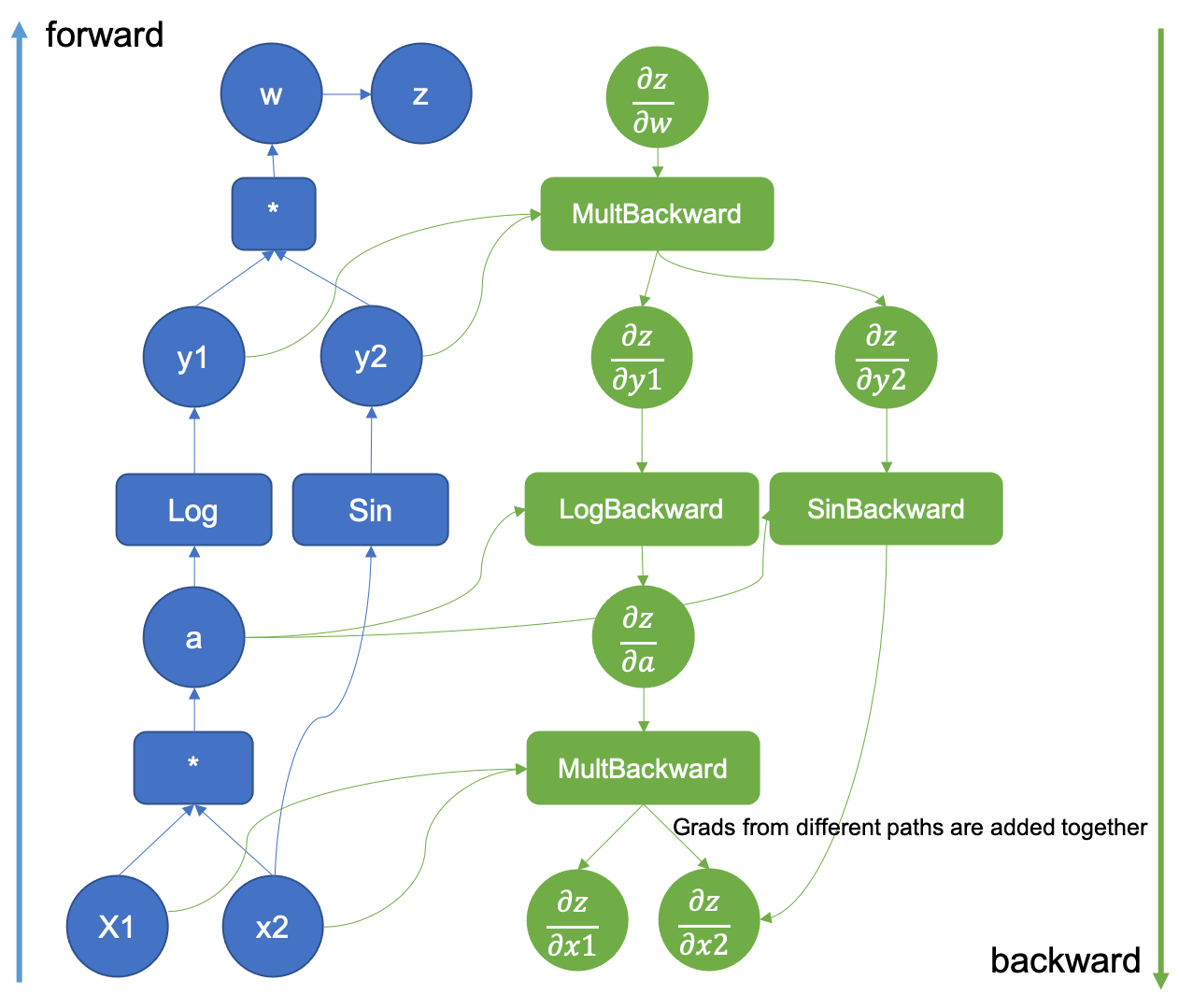
You can observe the information stored by PyTorch during the forward pass by accessing the grad_fn attribute of a tensor. To access the gradients of a tensor, you can use the grad attribute.
>>> a = torch.tensor([1,2,3], dtype=torch.float, requires_grad=True)
>>> b = torch.tensor([1,0,1], dtype=torch.float)
>>> c = (a+b).mean()
>>> c
tensor(2.6667, grad_fn=<MeanBackward0>)
>>>
>>> c.backward()                    # The gradients become available after calling the backward method
>>> a.grad
tensor([0.3333, 0.3333, 0.3333])
The example below shows how to compute gradients for all the weights of the nn.Module used to compute the prediction for which the loss is computed:
>>> import torch
>>>
>>> model = torch.nn.Linear(3, 1)
>>> optimizer = torch.optim.SGD(model.parameters(), lr=0.01)
>>>
>>> x = torch.tensor([1, 2, 3], dtype=torch.float32)
>>> y = model(x)
>>>
>>> loss = torch.nn.functional.mse_loss(y, torch.tensor([1.]))
>>> loss.backward()
>>>
>>> model.weight.grad
tensor([[0.2462, 0.4925, 0.7387]])
3.7.2 - Weight Update
In PyTorch, the update of the model weights based on the gradients computed during backpropagation is made using the step method of the optimizer.
Usually, before calling the backward method on the loss, you call the zero_grad method of the optimizer, to ensure previous gradients are set to 0. However, in some cases, gradient accumulation might be useful. For example, when your model is affected by the batch size and you can't fit a big enough batch in GPU memory, it can be useful to split the batch into N smaller batches, and then accumulate the gradient for N batches before updating the weights.
Below is an example of the usage of the step and zero_grad methods:
import torch

model = torch.nn.Linear(3, 1)
optimizer = torch.optim.SGD(model.parameters(), lr=0.01)

x = torch.tensor([1, 2, 3], dtype=torch.float32)

for i in range(10):
    y = model(x)
    loss = torch.nn.functional.mse_loss(y, torch.tensor([1.]))
    optimizer.zero_grad()
    loss.backward()
    optimizer.step()
To better understand how the gradients are computed, we highly recommend reading the Autograd mechanics (opens in a new tab) and How Computational Graphs are Constructed in PyTorch (opens in a new tab) guides in the PyTorch documentation.